吴恩达

# Neural Network

• Example: House Price Prediction

Standard Neural Network, CNN (convolutional, 图像等), RNN (recurrent, 时序序列)

Structured Data: 表格数据
Unstructured Data: 文本，语音，视频，图片

为什么效果好？
scale of data + scale of computation + better algorithms

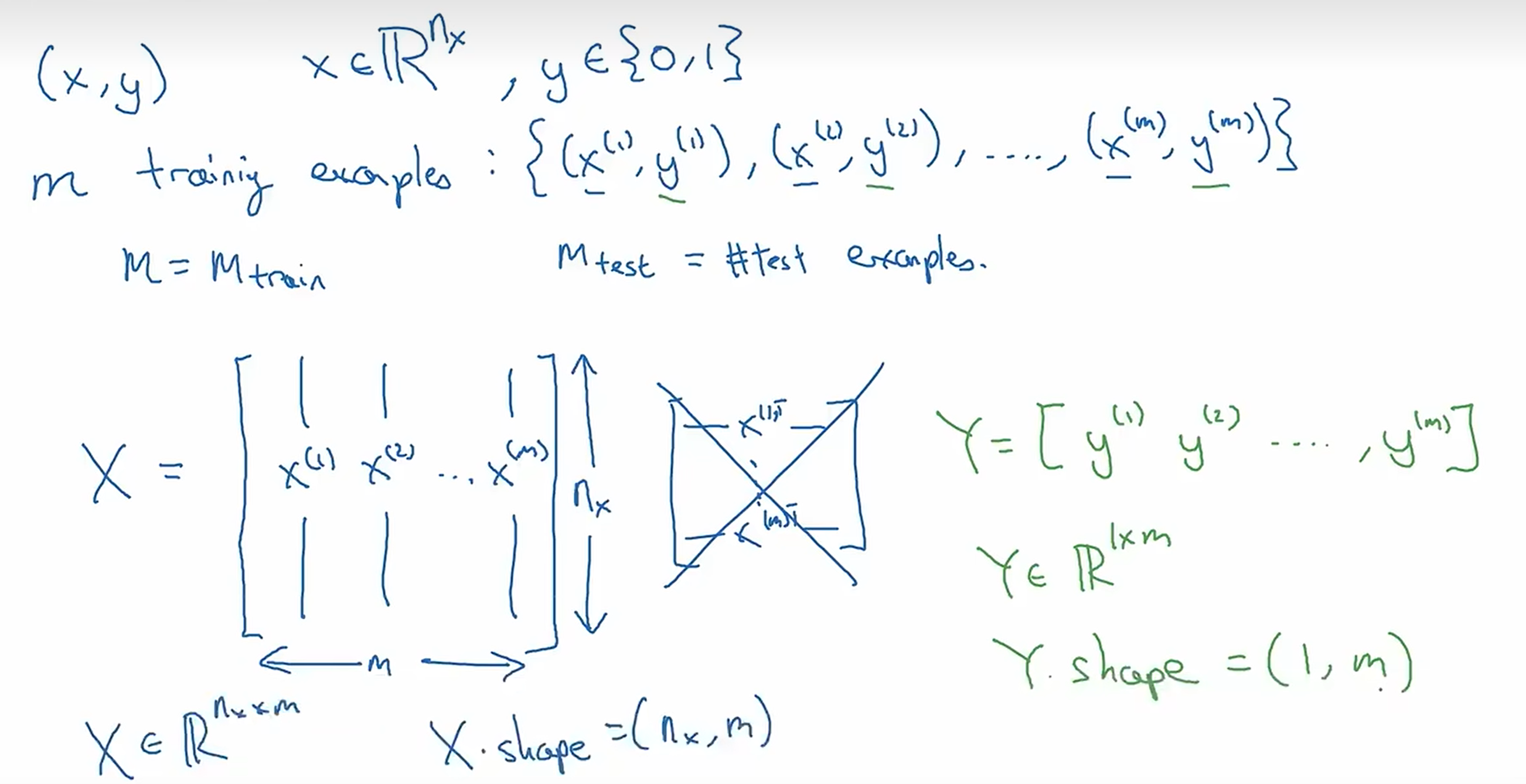
# Basic of NN

# Binary Classification

输入 x 输出 0 或 1

对于训练集，有 m 个样本
m 个输入向量组成$n_x \times m$ 的矩阵 X
m 个 label 组成$1 \times m$ 的行向量 Y

# Logistic Regression

一种二分类算法
given x, want $\hat{y} = P(y=1|x), x \in \mathbb{R}^n$
Parameters: weights w, bias b
Output: $\hat{y} = \sigma(w^Tx + b)$

$w$ 是一个列向量，大小为 $n_x \times 1$，解释是对于每个特征都有一个权重
$\sigma(z) = \frac{1}{1+e^{-z}}$ (sigmoid function, make sure $\hat{y} \in [0, 1]$)

1
2

def basic_sigmoid(x):
    return 1/(1 + math.exp(-x))

1
2

def basic_sigmoid(x):
    return 1/(1 + np.exp(-x))

1
2
3
4

def sigmoid_derivative(x):
    s = sigmoid(x)
    ds = s(1 - s)
    return ds

# Logistic Regression Cost Function

Given${(x^(1), y^(1)), ..., (x^(m), y^(m))}$, want $\hat{y}^{(i)} \approx y^{(i)}$
希望预测值和真实值接近
Loss function: 对于一个样本来说
$L(\hat{y}, y) = -[y \log(\hat{y}) + (1-y) \log(1-\hat{y})]$
不希望有多个局部最优，所以用交叉熵损失函数
Cost function: 对于$m$ 个样本（整个训练集）来说

$$J(w, b) = \frac{1}{m} \sum_{i=1}^m L(\hat{y}^{(i)}, y^{(i)}) = -\frac{1}{m} \sum_{i=1}^m [y^{(i)} \log(\hat{y}^{(i)}) + (1-y^{(i)}) \log(1-\hat{y}^{(i)})]$$

找到一组参数$w,b$ 使得$J(w,b)$ 最小

# Gradient Descent

梯度下降
为了便于理解，先忽略 b，只考虑 w，对于$J(w)$:

$$repeat \{ w := w - \alpha \frac{\partial J(w)}{\partial w} \}$$

$\alpha$ 是学习率，也就是一次迭代所使用的步长，正负取决于初始值在哪边

对于$J(w, b)$

$$repeat \{ w := w - \alpha \frac{\partial J(w, b)}{\partial w} b := b - \alpha \frac{\partial J(w, b)}{\partial b} \}$$

Derivative 表示函数的变化率，Gradient 表示多变量函数的变化率方向和大小

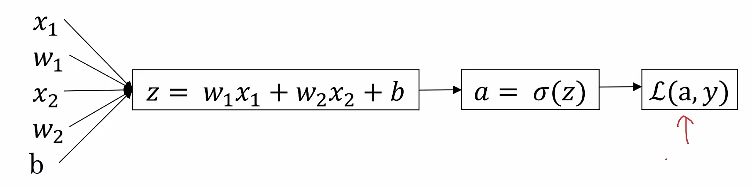
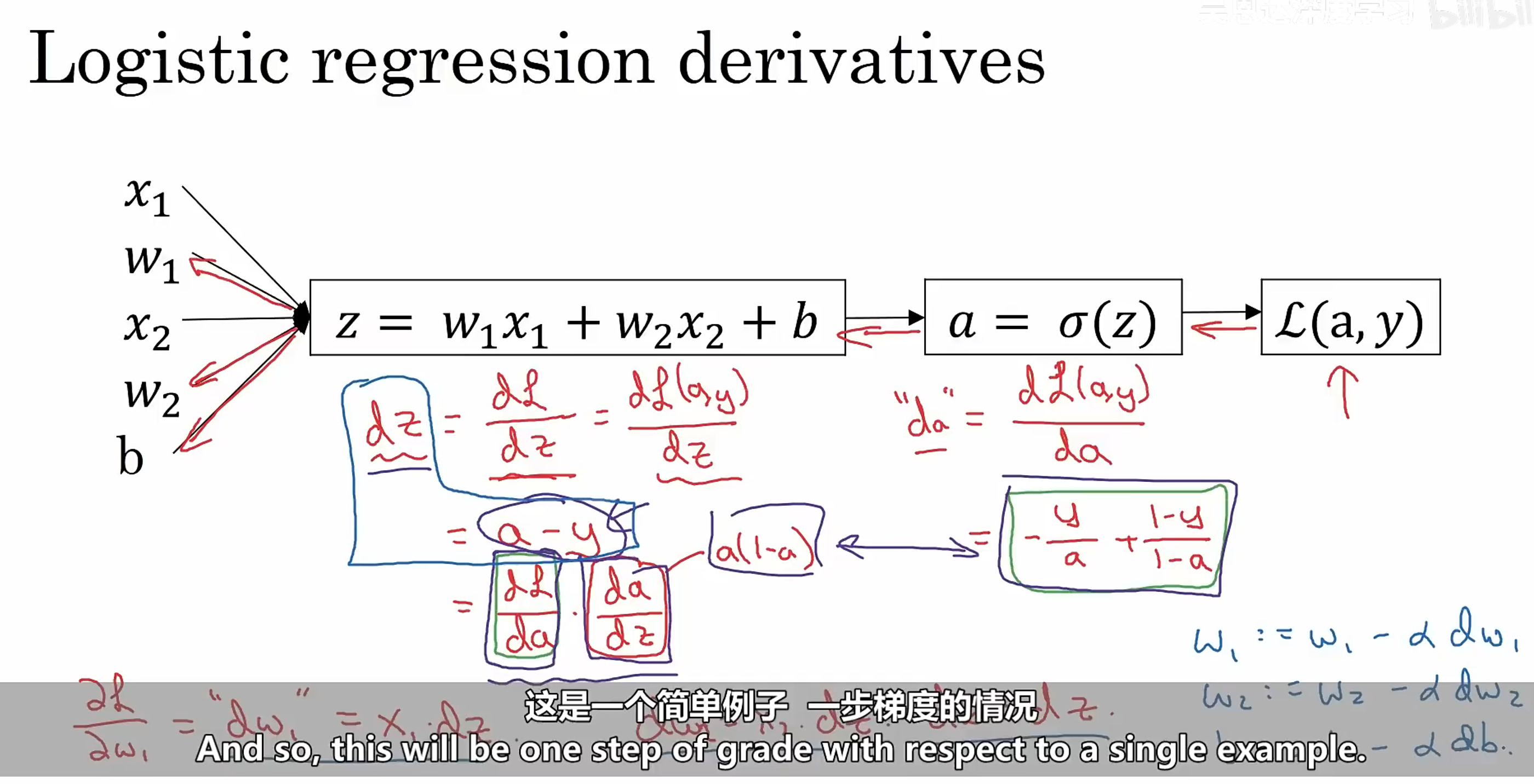
# Logistic Regression Gradient Descent

在一个样本上：

采用链式求导，先用$L(a, y)$ 对$a$ 求导

$$\frac{\partial L}{\partial a} = -\frac{y}{a} + \frac{1-y}{1-a}$$

再用$a$ 对$z$ 求导 (sigmoid 函数求导)

$$\frac{\partial L}{\partial z} = \frac{\partial L}{\partial a} \cdot \frac{\partial a}{\partial z} = -\frac{y}{a} + \frac{1-y}{1-a} \cdot a(1-a) = a - y$$

再用$z$ 对$w$ 求导

$$z = w^Tx + b = w_1 x_1 + w_2 x_2 + ... + w_n x_n + b 所以\frac{\partial z}{\partial w_i} = x_i$$

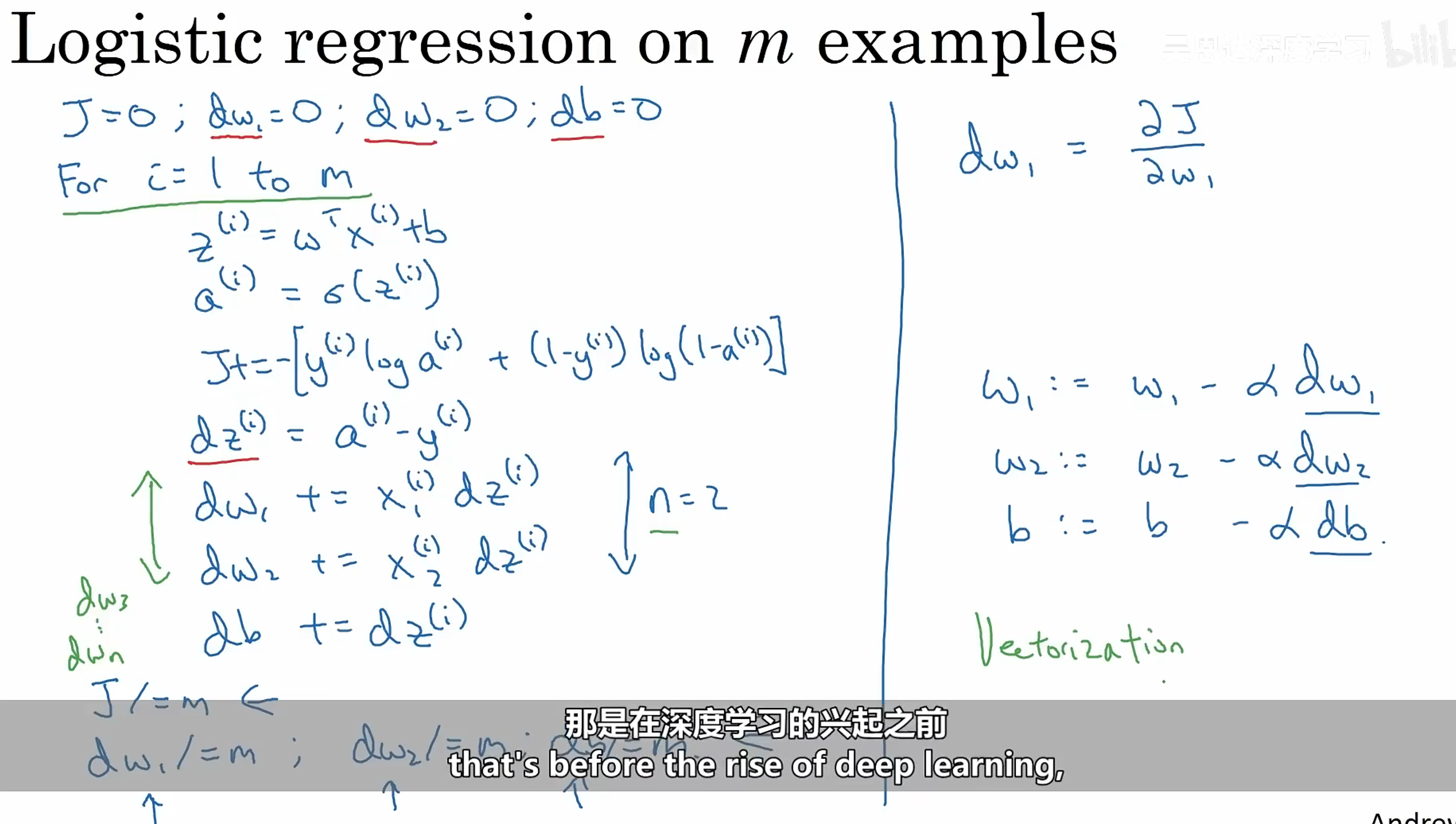
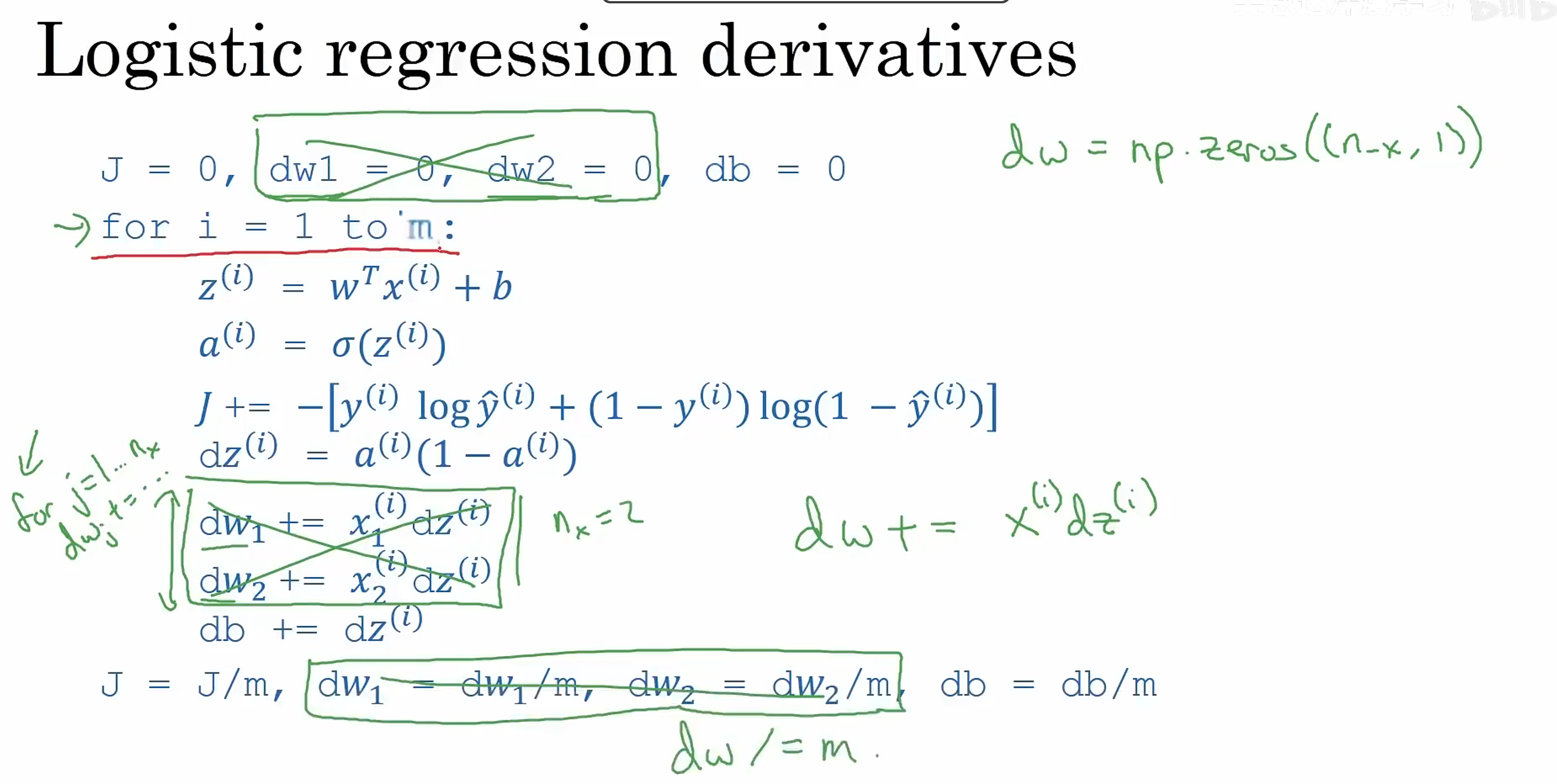
# Logistic Regression Gradient Descent on m samples

对于 m 个样本：

$$J(w, b) = \frac{1}{m} \sum_{i=1}^m L(a^{(i)}, y^{(i)}) where a^{(i)} = \sigma(z^{(i)}) = \sigma(w^Tx^{(i)} + b)$$

串行的话只能用 for 循环，但是太慢了，所以可以利用矩阵运算

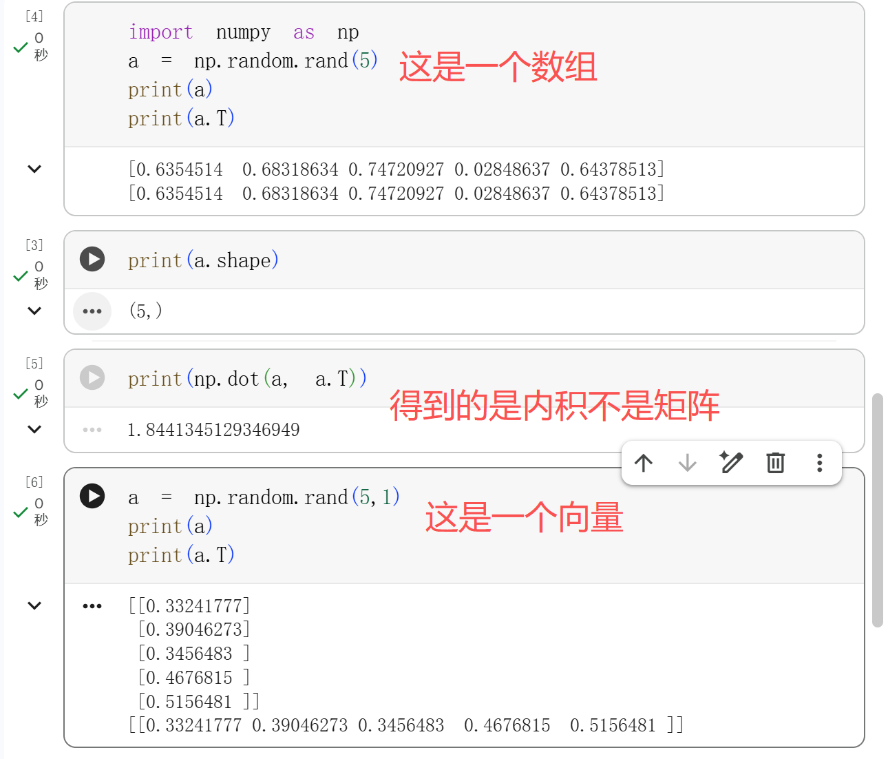
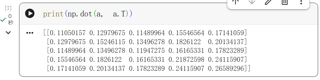
# Vectorization

向量化
Avoid explicit for-loops, use matrix/vector operations instead

$$u = Av u_i = \sum_{j=1}^n A_{ij} v_j$$

1

u = np.dot(A, v)

给定一个列向量 v

$$v^T = [v_1, v_2, ..., v_n]$$

对 v 中每个元素做指数运算

$$u^T = [e^{v_1}, e^{v_2}, ..., e^{v_n}]$$

1
2
3

u = np.zeros((n,1))
for i in range(n):
    u[i] = np.exp(v[i])

改进为:

1
2

u = np.exp(v)
# np.log(), np.sum(), np.mean(), np.abs(), np.maximum(v,0)...

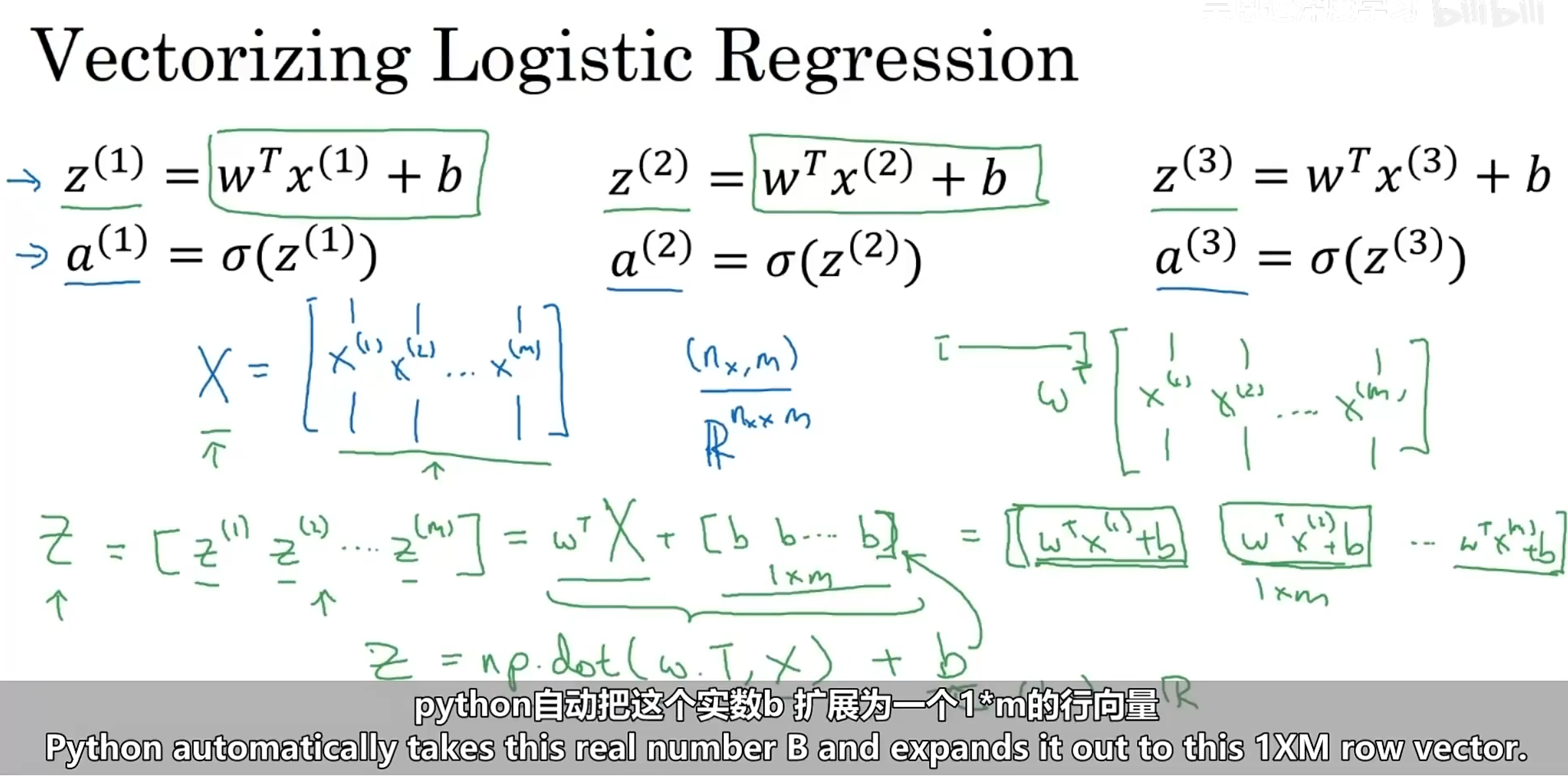
# Vectorization for Logistic Regression

对于逻辑回归，尝试移除一个 for 循环

但对于 m 个样本，仍然需要循环 m 次
尝试移除所有 for 循环：

1
2

Z = np.dot(w.T, X) + b  # shape (1, m)
A = 1 / (1 + np.exp(-Z))  # shape (1, m)

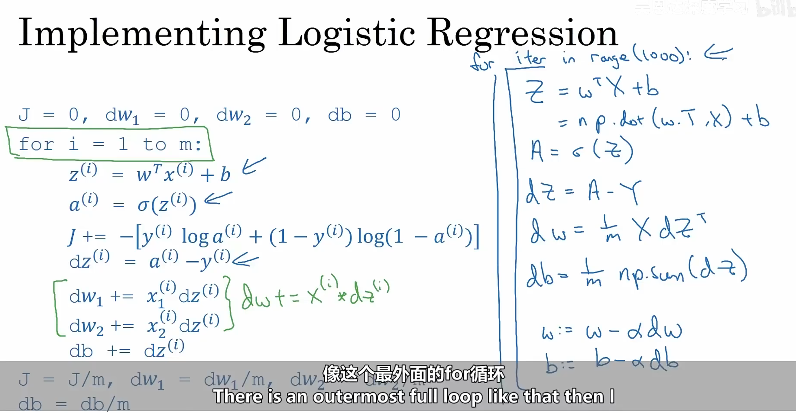
# Vectorized Logistic Regression’s Gradient Computation

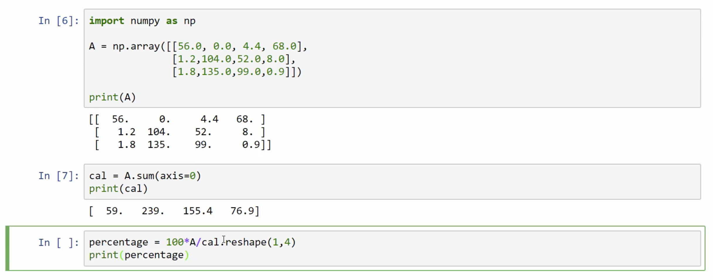
# Broadcasting in python

广播机制

axis 参数指定广播的方向:
axis = 0 : 垂直方向
axis = 1 : 水平方向

python/numpy:


计算的话最好全部用向量，不要用数组，不然会出问题

1
2

x_norm = np.linalg.norm(x, axis=1, keepdims=True)
x = x / x_norm

# 用 numpy 实现 softmax

用于多分类

$$\text{for } x \in \mathbb{R}^{1\times n} \text{, } softmax(x) = softmax(\begin{bmatrix} x_1 && x_2 && ... && x_n \end{bmatrix}) = \begin{bmatrix} \frac{e^{x_1}}{\sum_{j}e^{x_j}} && \frac{e^{x_2}}{\sum_{j}e^{x_j}} && ... && \frac{e^{x_n}}{\sum_{j}e^{x_j}} \end{bmatrix}$$

$$\text{For a matrix } x \in \mathbb{R}^{m \times n}, \text{ let } x_{ij} \text{ denote the element in the } i\text{-th row and } j\text{-th column.}$$

$$softmax(x) = softmax\begin{bmatrix} x_{11} & x_{12} & x_{13} & \dots & x_{1n} \\ x_{21} & x_{22} & x_{23} & \dots & x_{2n} \\ \vdots & \vdots & \vdots & \ddots & \vdots \\ x_{m1} & x_{m2} & x_{m3} & \dots & x_{mn} \end{bmatrix} = \begin{bmatrix} \frac{e^{x_{11}}}{\sum_{j}e^{x_{1j}}} & \frac{e^{x_{12}}}{\sum_{j}e^{x_{1j}}} & \frac{e^{x_{13}}}{\sum_{j}e^{x_{1j}}} & \dots & \frac{e^{x_{1n}}}{\sum_{j}e^{x_{1j}}} \\ \frac{e^{x_{21}}}{\sum_{j}e^{x_{2j}}} & \frac{e^{x_{22}}}{\sum_{j}e^{x_{2j}}} & \frac{e^{x_{23}}}{\sum_{j}e^{x_{2j}}} & \dots & \frac{e^{x_{2n}}}{\sum_{j}e^{x_{2j}}} \\ \vdots & \vdots & \vdots & \ddots & \vdots \\ \frac{e^{x_{m1}}}{\sum_{j}e^{x_{mj}}} & \frac{e^{x_{m2}}}{\sum_{j}e^{x_{mj}}} & \frac{e^{x_{m3}}}{\sum_{j}e^{x_{mj}}} & \dots & \frac{e^{x_{mn}}}{\sum_{j}e^{x_{mj}}} \end{bmatrix} = \begin{pmatrix} softmax\text{(first row of x)} \\ softmax\text{(second row of x)} \\ ... \\ softmax\text{(last row of x)} \\ \end{pmatrix}$$

1
2
3
4

def softmax(x):
    x_exp = np.exp(x)
    s = np.sum(x_exp, asix = 1, keepdims = True)
    return x_exp / s

# Logistic Regression’s Cost Function

$$if y = 1: p(y|x) = \hat{y} if y = 0: p(y|x) = 1 - \hat{y}$$

解释：p (y|x) 是模型预测正确的概率，在已知输入 x 的情况下，真实标签 y 出现的概率
把这个概率代入 交叉熵损失函数（Cross-Entropy Loss）

$$L(\hat{y}, y) = -[y \log(\hat{y}) + (1-y) \log(1-\hat{y})]$$

就是损失函数

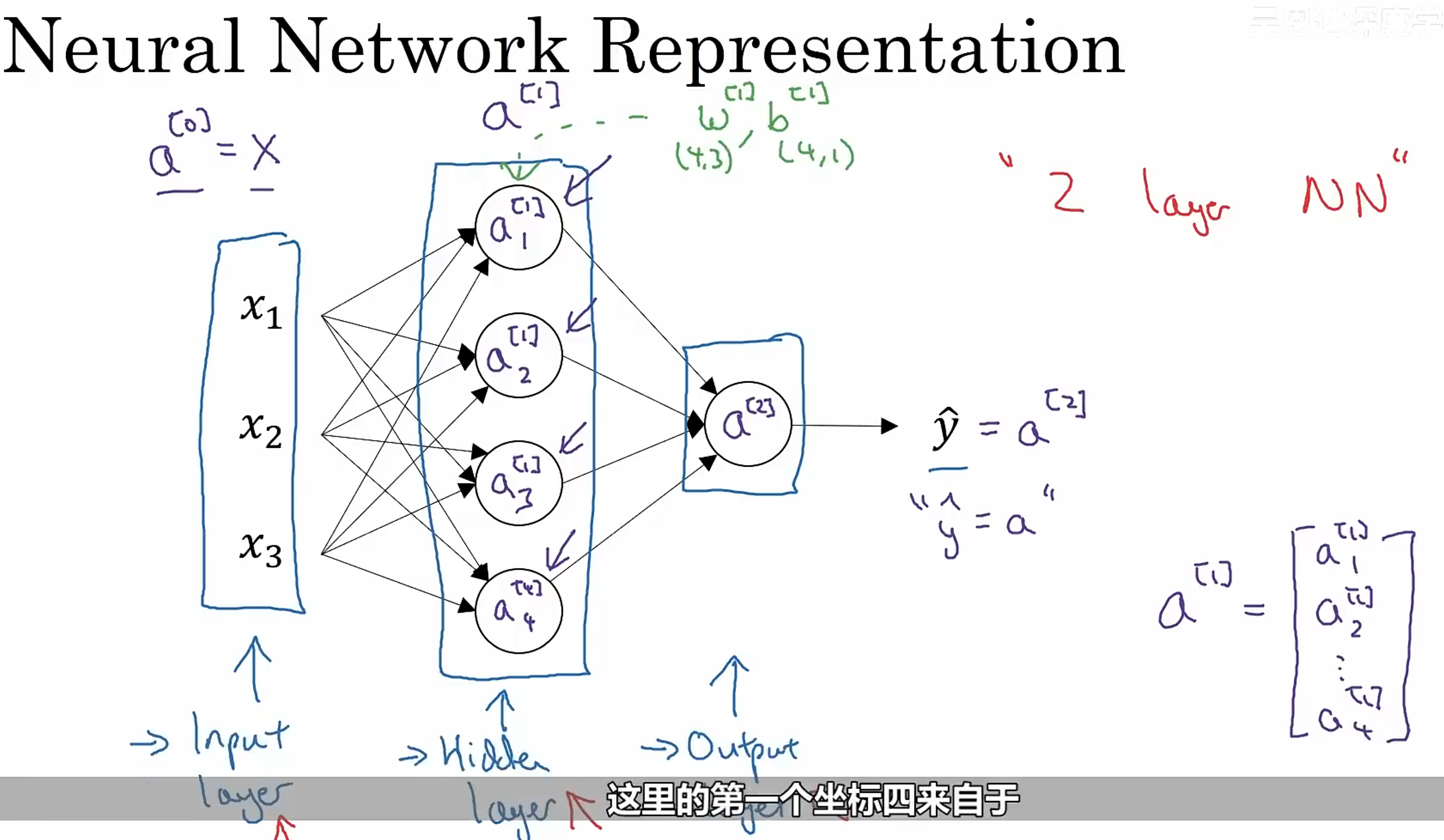
# Neural Network Overview

# Neural Network Representation

单隐藏层的 NN：
分别用$a^{[0]}$ 表示输入层，$a^{[1]}$ 表示隐藏层，$a^{[2]}$ 表示输出层

# Computing a Neural Network’s Output

一个带两层隐藏层的神经网络，最后用 Sigmoid 输出

# Vectorizing across multiple examples